
| 일 | 월 | 화 | 수 | 목 | 금 | 토 |
|---|---|---|---|---|---|---|
| 1 | 2 | 3 | ||||
| 4 | 5 | 6 | 7 | 8 | 9 | 10 |
| 11 | 12 | 13 | 14 | 15 | 16 | 17 |
| 18 | 19 | 20 | 21 | 22 | 23 | 24 |
| 25 | 26 | 27 | 28 | 29 | 30 | 31 |
- 회귀 알고리즘 평가
- 학습용데이터
- 데이터 분리
- 분류 머신러닝 모델
- 데이터 전 처리
- 지니 불순도
- 뉴런 신경망
- ICDL 파이썬
- LinearRegression 모델
- 더미 기법
- 알고리즘 기술
- 딥러닝 역사
- 결측값 처리
- 불순도
- 수치형 자료
- 스케이링
- 수치 맵핑 기법
- 경사하강법
- 다중선형 회귀
- 가중치 업데이트
- 머신러닝 과정
- 퍼셉트론
- MSEE
- 명목형
- 지도학습 분류
- 항공지연
- 웹 크롤링
- 평가용 데이터
- 이상치 처리
- 지도학습
- Today
- Total
끄적이는 기록일지
[머신러닝] 07.다양한 신경망_(2) 자연어 처리를 위한 전처리, 딥러닝 모델 본문
[머신러닝] 07.다양한 신경망_(1) 이미지 처리를 위한 전처리, 딥러닝 모델
[머신러닝] 06.텐서플로와 신경망_(1) 딥러닝 모델의 학습 방법 1. 딥러닝 모델 전 시간 다층 퍼셉트론까지 이야기했습니다. 모델 안에 은닉층이 많아진다면, 깊은 신경망이라는 의미의 Deep Learning
kcy51156.tistory.com
1. 자연어 처리 예시

2. 자연어 처리를 위한 데이터 전 처리
1. 오류교정(Noise Canceling) : 자연어 문장의 스펠링체크및띄어쓰기오류교정
안녕 하세요. 반갑 스니다. -> 안녕하세요. 반갑습니다.2. 토큰화(Tokenizing) : 문장을 토큰(Token)으로 나눔, 토큰은 어절, 단어 등으로 목적에 따라 다르게 정의
“딥러닝 기초 과목 수강하고 있습니다.” => ['딥', '러닝', '기초', '과목', '을', '수강', '하고', '있습니다', '.']3. 불용어 제거(StopWordremoval) : 불필요한 단어를 의미하는 불용어(StopWord)제거
한국어stopword예시)
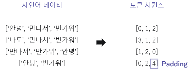
아, 휴, 아이구, 아이쿠, 아이고, 쉿, 그렇지않으면, 그러나, 그런데, 하지만, ...4. Bag of Words : 자연어 데이터에 속해 있는 단어들의 가방

5. 토큰 시퀀스 : Bag of words에서 단어에 해당되는 인덱스로 변환. 모든 문장의 길이를 맞추기 위해 기준보다 짧은 문장에는 패딩을 수행
3. 자연어 처리를 위한 딥러닝 모델
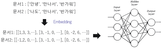
1. 워드 임베딩(Word Embedding)의 정의 : 단순하게 Bag of Words의 인덱스로 정의된 토큰들에게 의미를 부여하는 방식

2. 기존 다층 퍼셉트론 신경망의 자연어 분류 방식 : 자연어 문장을 기존 MLP모델에 적용시키기에는 한계가 있음
토큰간의 순서와 관계를 적용할 수 있는 모델은 없을까?
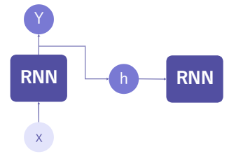
3. 자연어 분류를 위한 순환 신경망(Recurrent Neural Network) : 기존 퍼셉트론 계산과 비슷하게 X 입력 데이터를 받아 Y를 출력

4. 순환 신경망의 입출력 구조 : 출력값을 두갈래로 나뉘어 신경망에게 ‘기억’하는 기능을 부여
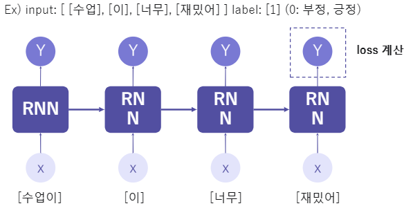
- 순환 신경망 기반 자연어 분류 예시
4. 정리

임베딩은 토큰의 특징을 찾아내고, RNN 이전 토큰의 영향을 받으며 학습한다.
- 순환 신경망 기반 다양한 자연어 처리 기술

5. 실습
영화 리뷰 긍정/부정 분류 RNN 모델 - 데이터 전 처리
이번 실습에서는 영화 리뷰 데이터를 바탕으로 감정 분석을 하는 모델을 학습 시켜 보겠습니다. 영화 리뷰와 같은 자연어 자료는 곧 단어의 연속적인 배열로써, 시계열 자료라고 볼 수 있습니다. 즉, 시계열 자료(연속된 단어)를 이용해 리뷰에 내포된 감정(긍정, 부정)을 예측하는 분류기를 만들어 보겠습니다.
데이터셋은 IMDB 영화 리뷰 데이터 셋을 사용합니다. 훈련용 5,000개와 테스트용 1,000개로 이루어져 있으며, 레이블은 긍정/부정으로 두 가지입니다. 우선 자연어 데이터를 RNN 모델의 입력으로 사용할 수 있도록 데이터 전 처리를 수행해보겠습니다.
RNN을 위한 자연어 데이터 전 처리
RNN의 입력으로 사용하기 위해서는 자연어 데이터는 토큰화 및 여러 가지의 데이터 처리가 필요합니다. 아래와 같이 자연어 데이터가 준비되어 있다면 마지막으로 패딩을 수행하여 데이터의 크기를 통일해야합니다.
1. 인덱스로 변환된 X_train, X_test 시퀀스에 패딩을 수행하고 각각 X_train, X_test에 저장합니다.
- 시퀀스 최대 길이는 300으로 설정합니다.
sequence.pad_sequences(data, maxlen=300, padding='post'): data 시퀀스의 크기가 maxlen인자보다 작으면 그 크기에 맞게 패딩을 추가합니다.
Keras에서 RNN 모델을 만들기 위해 필요한 함수/라이브러리
일반적으로 RNN 모델은 입력층으로 Embedding 레이어를 먼저 쌓고, RNN 레이어를 몇 개 쌓은 다음, 이후 Dense 레이어를 더 쌓아 완성합니다.
2. RNN 모델을 구현합니다.
- 임베딩 레이어 다음으로 SimpleRNN을 사용하여 RNN 레이어를 쌓고 노드의 개수는 5개로 설정합니다.
#임베딩 레이어
tf.keras.layers.Embedding(input_dim, output_dim, input_length)
: 들어온 문장을 단어 임베딩(embedding)하는 레이어
- input_dim: 들어올 단어의 개수
- output_dim: 결과로 나올 임베딩 벡터의 크기(차원)
- input_length: 들어오는 단어 벡터의 크기
#RNN 레이어
tf.keras.layers.SimpleRNN(units)
: 단순 RNN 레이어
- units: 레이어의 노드 수
3. evaluate 메서드를 사용하여 평가용 데이터를 활용하여 모델을 평가합니다.
- loss와 accuracy를 계산하고 loss, test_acc에 저장합니다.
model.evaluate(X, Y)- evaluate() 메서드는 학습된 모델을 바탕으로 입력한 feature 데이터 X와 label Y의 loss 값과 metrics 값을 출력합니다.
4. predict 메서드를 사용하여 평가용 데이터에 대한 예측 결과를 predictions에 저장합니다.
model.predict(X)- X 데이터의 예측 label 값을 출력합니다.
# data_process.py
import json
import numpy as np
import tensorflow as tf
from keras.datasets import imdb
from keras.preprocessing import sequence

import logging, os
logging.disable(logging.WARNING)
os.environ["TF_CPP_MIN_LOG_LEVEL"] = "3"

np_load_old = np.load
np.load = lambda *a,**k: np_load_old(*a, allow_pickle=True, **k)

# 데이터를 불러오고 전처리하는 함수입니다.

n_of_training_ex = 5000
n_of_testing_ex = 1000

PATH = "./data/"

def imdb_data_load():

    X_train = np.load(PATH + "X_train.npy")[:n_of_training_ex]
    y_train = np.load(PATH + "y_train.npy")[:n_of_training_ex]
    X_test = np.load(PATH + "X_test.npy")[:n_of_testing_ex]
    y_test = np.load(PATH + "y_test.npy")[:n_of_testing_ex]

    # 단어 사전 불러오기
    with open(PATH+"imdb_word_index.json") as f:
        word_index = json.load(f)
    # 인덱스 -> 단어 방식으로 딕셔너리 설정
    inverted_word_index = dict((i, word) for (word, i) in word_index.items())
    # 인덱스를 바탕으로 문장으로 변환
    decoded_sequence = " ".join(inverted_word_index[i] for i in X_train[0])


    print("첫 번째 X_train 데이터 샘플 문장: \n",decoded_sequence)
    print("\n첫 번째 X_train 데이터 샘플 토큰 인덱스 sequence: \n",X_train[0])
    print("첫 번째 X_train 데이터 샘플 토큰 시퀀스 길이: ", len(X_train[0]))
    print("첫 번째 y_train 데이터: ",y_train[0])

    return X_train, y_train, X_test, y_test
import json
import numpy as np
import tensorflow as tf
import data_process
from keras.datasets import imdb
from keras.preprocessing import sequence
import logging, os
logging.disable(logging.WARNING)
os.environ["TF_CPP_MIN_LOG_LEVEL"] = "3"
# 동일한 실행 결과 확인을 위한 코드입니다.
np.random.seed(123)
tf.random.set_seed(123)
# 학습용 및 평가용 데이터를 불러오고 샘플 문장을 출력합니다.
X_train, y_train, X_test, y_test = data_process.imdb_data_load()
"""
1. 인덱스로 변환된 X_train, X_test 시퀀스에 패딩을 수행하고 각각 X_train, X_test에 저장합니다.
시퀀스 최대 길이는 300으로 설정합니다.
"""
X_train = sequence.pad_sequences(X_train, maxlen=300, padding='post')
X_test = sequence.pad_sequences(X_test, maxlen=300, padding='post')
print("\n패딩을 추가한 첫 번째 X_train 데이터 샘플 토큰 인덱스 sequence: \n",X_train[0])
embedding_vector_length = 32
"""
2. 모델을 구현합니다.
임베딩 레이어 다음으로 `SimpleRNN`을 사용하여 RNN 레이어를 쌓고 노드의 개수는 5개로 설정합니다.
Dense 레이어는 0, 1 분류이기에 노드를 1개로 하고 activation을 'sigmoid'로 설정되어 있습니다.
"""
model = tf.keras.models.Sequential([
tf.keras.layers.Embedding(1000, embedding_vector_length, input_length = max_review_length),
tf.keras.layers.SimpleRNN(5),
tf.keras.layers.Dense(1, activation='sigmoid')
])
# 모델을 확인합니다.
print(model.summary())
# 학습 방법을 설정합니다.
model.compile(loss = 'binary_crossentropy', optimizer = 'adam', metrics = ['accuracy'])
# 학습을 수행합니다.
model_history = model.fit(X_train, y_train, epochs = 5, verbose = 2)
"""
3. 평가용 데이터를 활용하여 모델을 평가합니다.
loss와 accuracy를 계산하고 loss, test_acc에 저장합니다.
"""
loss, test_acc = model.evaluate(X_test, y_test, verbose = 0)
"""
4. 평가용 데이터에 대한 예측 결과를 predictions에 저장합니다.
"""
predictions = model.predict(X_test)
# 모델 평가 및 예측 결과를 출력합니다.
print('\nTest Loss : {:.4f} | Test Accuracy : {}'.format(loss, test_acc))
print('예측한 Test Data 클래스 : ',1 if predictions[0]>=0.5 else 0)
>>> 첫 번째 X_train 데이터 샘플 문장:
the as you with out themselves powerful and and their becomes and had and of lot from anyone to have after out atmosphere never more room and it so heart shows to years of every never going and help moments or of every and and movie except her was several of enough more with is now and film as you of and and unfortunately of you than him that with out themselves her get for was and of you movie sometimes movie that with scary but and to story wonderful that in seeing in character to of and and with heart had and they of here that with her serious to have does when from why what have and they is you that isn't one will very to as itself with other and in of seen over and for anyone of and br and to whether from than out themselves history he name half some br of and and was two most of mean for 1 any an and she he should is thought and but of script you not while history he heart to real at and but when from one bit then have two of script their with her and most that with wasn't to with and acting watch an for with and film want an
첫 번째 X_train 데이터 샘플 토큰 인덱스 sequence:
[1, 14, 22, 16, 43, 530, 973, 2, 2, 65, 458, 2, 66, 2, 4, 173, 36, 256, 5, 25, 100, 43, 838, 112, 50, 670, 2, 9, 35, 480, 284, 5, 150, 4, 172, 112, 167, 2, 336, 385, 39, 4, 172, 2, 2, 17, 546, 38, 13, 447, 4, 192, 50, 16, 6, 147, 2, 19, 14, 22, 4, 2, 2, 469, 4, 22, 71, 87, 12, 16, 43, 530, 38, 76, 15, 13, 2, 4, 22, 17, 515, 17, 12, 16, 626, 18, 2, 5, 62, 386, 12, 8, 316, 8, 106, 5, 4, 2, 2, 16, 480, 66, 2, 33, 4, 130, 12, 16, 38, 619, 5, 25, 124, 51, 36, 135, 48, 25, 2, 33, 6, 22, 12, 215, 28, 77, 52, 5, 14, 407, 16, 82, 2, 8, 4, 107, 117, 2, 15, 256, 4, 2, 7, 2, 5, 723, 36, 71, 43, 530, 476, 26, 400, 317, 46, 7, 4, 2, 2, 13, 104, 88, 4, 381, 15, 297, 98, 32, 2, 56, 26, 141, 6, 194, 2, 18, 4, 226, 22, 21, 134, 476, 26, 480, 5, 144, 30, 2, 18, 51, 36, 28, 224, 92, 25, 104, 4, 226, 65, 16, 38, 2, 88, 12, 16, 283, 5, 16, 2, 113, 103, 32, 15, 16, 2, 19, 178, 32]
첫 번째 X_train 데이터 샘플 토큰 시퀀스 길이: 218
첫 번째 y_train 데이터: 1
패딩을 추가한 첫 번째 X_train 데이터 샘플 토큰 인덱스 sequence:
[ 1 14 22 16 43 530 973 2 2 65 458 2 66 2 4 173 36 256
5 25 100 43 838 112 50 670 2 9 35 480 284 5 150 4 172 112
167 2 336 385 39 4 172 2 2 17 546 38 13 447 4 192 50 16
6 147 2 19 14 22 4 2 2 469 4 22 71 87 12 16 43 530
38 76 15 13 2 4 22 17 515 17 12 16 626 18 2 5 62 386
12 8 316 8 106 5 4 2 2 16 480 66 2 33 4 130 12 16
38 619 5 25 124 51 36 135 48 25 2 33 6 22 12 215 28 77
52 5 14 407 16 82 2 8 4 107 117 2 15 256 4 2 7 2
5 723 36 71 43 530 476 26 400 317 46 7 4 2 2 13 104 88
4 381 15 297 98 32 2 56 26 141 6 194 2 18 4 226 22 21
134 476 26 480 5 144 30 2 18 51 36 28 224 92 25 104 4 226
65 16 38 2 88 12 16 283 5 16 2 113 103 32 15 16 2 19
178 32 0 0 0 0 0 0 0 0 0 0 0 0 0 0 0 0
0 0 0 0 0 0 0 0 0 0 0 0 0 0 0 0 0 0
0 0 0 0 0 0 0 0 0 0 0 0 0 0 0 0 0 0
0 0 0 0 0 0 0 0 0 0 0 0 0 0 0 0 0 0
0 0 0 0 0 0 0 0 0 0 0 0]
Model: "sequential"
_________________________________________________________________
Layer (type) Output Shape Param #
=================================================================
embedding (Embedding) (None, 300, 32) 32000
_________________________________________________________________
simple_rnn (SimpleRNN) (None, 5) 190
_________________________________________________________________
dense (Dense) (None, 1) 6
=================================================================
Total params: 32,196
Trainable params: 32,196
Non-trainable params: 0
_________________________________________________________________
None
Train on 5000 samples
Epoch 1/5
5000/5000 - 11s - loss: 0.6936 - accuracy: 0.5048
Epoch 2/5
5000/5000 - 10s - loss: 0.6811 - accuracy: 0.5760
Epoch 3/5
5000/5000 - 10s - loss: 0.6664 - accuracy: 0.6102
Epoch 4/5
5000/5000 - 10s - loss: 0.6566 - accuracy: 0.6200
Epoch 5/5
5000/5000 - 9s - loss: 0.6167 - accuracy: 0.6886
Test Loss : 0.6145 | Test Accuracy : 0.703000009059906
예측한 Test Data 클래스 : 1
'AI실무' 카테고리의 다른 글
| [머신러닝] 07.다양한 신경망_(1) 이미지 처리를 위한 전처리, 딥러닝 모델 (0) | 2021.11.26 |
|---|---|
| [머신러닝] 06.텐서플로와 신경망_(2) 딥러닝 구현 (0) | 2021.10.15 |
| [머신러닝] 06.텐서플로와 신경망_(1) 딥러닝 모델의 학습 방법 (0) | 2021.10.15 |
| [딥러닝] 01.퍼셉트론_(2)퍼셉트론 (0) | 2021.10.08 |
| [딥러닝] 01.퍼셉트론_(1)딥러닝 (0) | 2021.10.08 |


